Mapping Gestures to Sound with a Neural Net

In this post, I want to discuss a slightly different usage for neural networks than has been explored so far. Rather than using neural nets to define relationships between strictly musical data (as in the previous post), here I will use them to define relationships between gestures and sounds.

Gesture recognition—the interpretation of human gestures by computers—is an important topic for the application of machine learning methods. Of course, what constitutes a “gesture” can vary widely depending on the context. In this post, I’ll be imagining the movement of a hand, fingertip, or other single point in a vertically oriented, two-dimensional plane. (Imagine tracing a shape on a steamed-up bathroom mirror.)

Just as in the previous post, I’ll use the ml.star library for Max developed by Benjamin Day Smith. You can download it through the Package Manager (File -> Show Package Manager). As before, we’ll also use a simple type of neural network called a multilayer perceptron (mlp), represented by the object [ml.mlp].

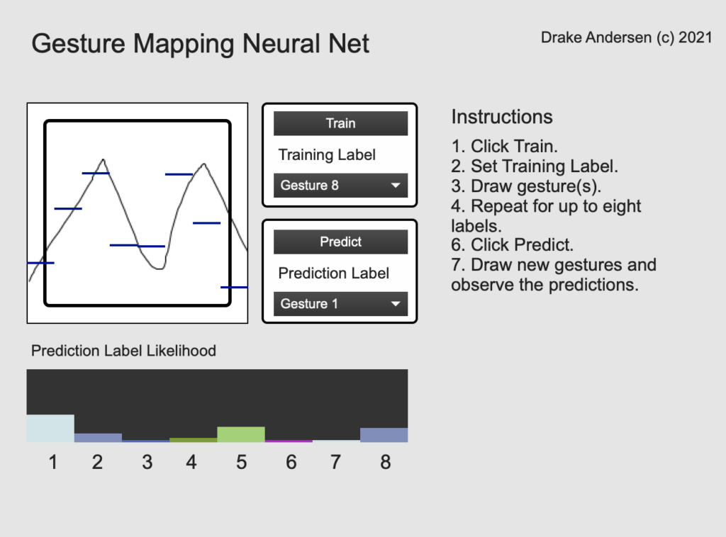
The basic idea for this patch is that each gesture will be represented as a list of numbers. When training the neural net, the user will specify a gesture label, which will then be associated with the particular sequence. I will use eight distinct labels, though this is easily modifiable. Over time, the idea is that the neural net can generalize what is distinctive about each gesture. Once the training is complete, the neural net will be able to categorize new gestures by assigning labels to the new gestures.

There are many different ways of defining gestures. For example, gestures can be dynamic (moving) or static (not moving). I’m especially interested in dynamic gestures, since their beginnings and endings can be recognized to automatically tell the computer when a gesture is starting or ending. To keep things simple, I will divide up the two-dimensional plane into eight columns and characterize each gesture according to the average values in these columns. (The fact that I have eight labels and eight columns is entirely coincidental—these do not have to be the same number.) The user will sweep their hand back and forth across the plane horizontally, with the variation in vertical position defining each gesture.

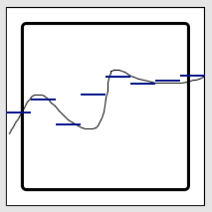
The image above illustrates a typical gesture, with the continuous human-generated gesture given by the black line, and the mean-based simplification given by the eight blue bars. (There is a slight horizontal discrepancy between the display position of the bars and the data segments they represent.)

Gesture recognition typically involves a lot of pre-processing because you have to transform human gestures—which are typically complex and time-based—into an input format that a neural network can recognize and work with. In this case, the eight vertical columns are the eight data points that make up the input layer of the neural network. The output layer will have eight points as well, but these will represent the eight possible gesture categories. These categories, it should be emphasized, will be completely user-defined: whatever the user labels “Gesture 1” will become gesture 1, etc.

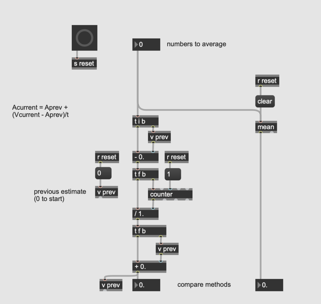
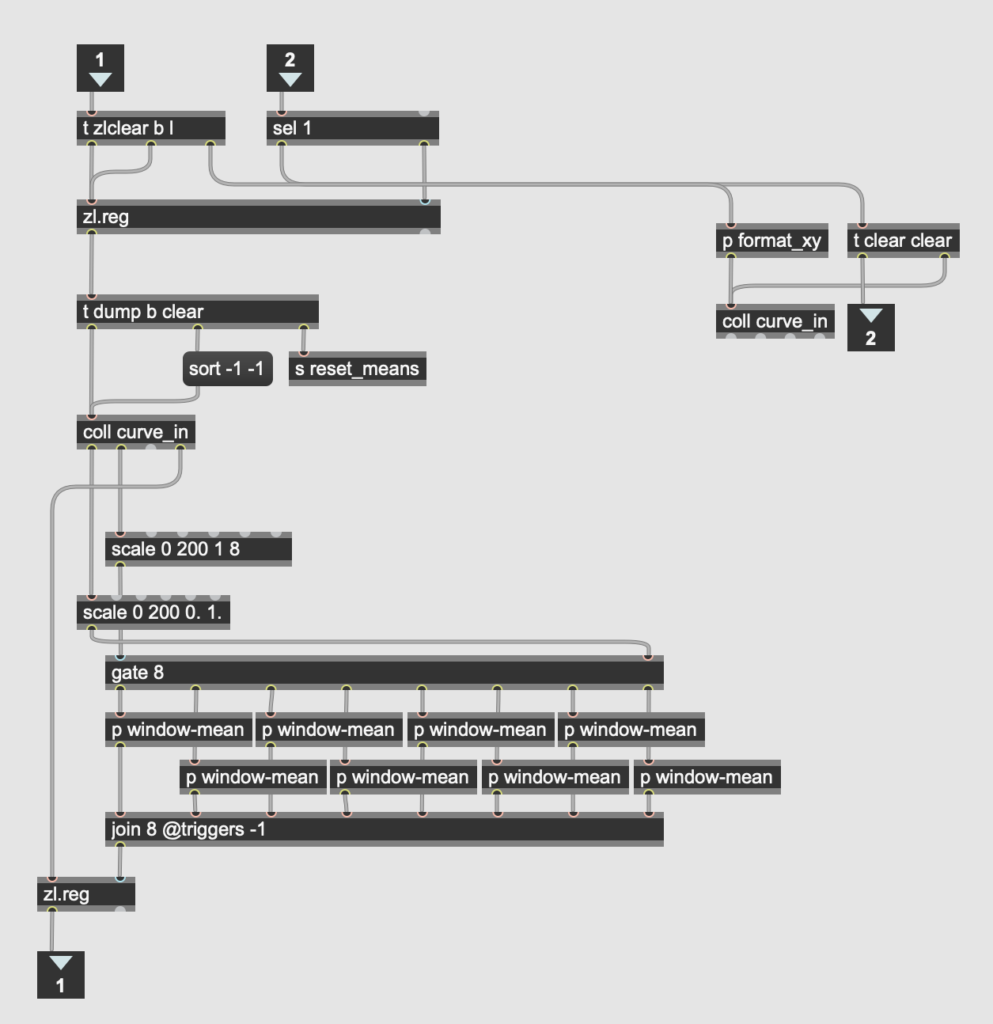
There were a handful of other minor processing details. For example, the [lcd] object used for drawing the line counts y values from the top down. In order to not confuse myself, I flipped this by running the xy coordinate list output through a [vexpr] object with a simple expression. I also had to calculate the mean of each segment separately, which involved sorting the values from the “dump” output of the coll object storing the line’s coordinates into eight bins of equal size. I ended up solving this in reasonably elegant fashion by scaling the x values to the range of one to eight and using them as the control for an 8-outlet gate, with each output leading to a separate [mean] object.

When in prediction mode, the patch gives not only the most likely label for a gesture, but also the likelihood for each label (as a multicolored [multislider] object). The final version of this patch, while functional and easy to use, also has plenty of room for improvement. For example, the inner workings of the neural net remain hidden to the user so as not to clutter the interface, but this also prevents the user from adjusting the inner structure to produce better predictions. The patch would also benefit from some gesture “filtering,” by which gestures are not recognized unless they pass across all eight columns. This will become especially important when we link it up with a computer vision system such as the LEAP motion in a later post.

Download the code bundle here.

Composing with a Neural Net

The first two blog posts in this series on machine learning and music covered some of the basic conceptual considerations for analyzing music through the use of neural networks. In this post, I want to explore the creative, generative possibilities of neural networks

Whereas I used Python in the previous two examples, in this example I’ll be using Max to get the audio side of things up and running more quickly. I’ll use a machine learning library for Max called ml.star, developed by Benjamin Day Smith. You can download it through the Package Manager (File -> Show Package Manager).

Just as with the analysis described in the previous post, it took me a little while to determine an application for machine learning in the compositional process that would be both manageable and interesting. In addition to these criteria, I wanted something that would function in real time (or close to it) and that would specifically use machine learning to simplify the choices and/or interface presented to the user, rather than overwhelming them with arcane parameters. I also imagined that a binary-encoded input layer would make things simple and easier to follow.

After some trial and error, I decided on developing a program to compose a drum sequence. However, instead of having the user input each sound individually (as with most sequencers), the user is presented with two phrases generated at random. They listen to the two phrases, and then click a button to indicate which they like better. If they prefer phrase #1, a new phrase #2 is generated, and vice versa. Over time, the idea is that the neural network will be able to infer the user’s preferences and generate phrases that more closely match the phrases the user has previously preferred.

I decided to use a very simple type of artificial neural network called a multilayer perceptron. A perceptron is a function that attempts to represent the relationship between its input and output by weighting corresponding nodes. While all perceptrons contain an input and output layer (the data to be evaluated and the evaluation, respectively), multilayer perceptrons are unique in that they contain one or more hidden layers that are weighted during the training phase. The ml.star package contains a multiplayer perception object called [ml.mlp].

After some experimentation, I finally settled on a structure for the program. Each drum phrase would be an eight-step sequence consisting of three instrumental parts (clap, kick, and hi-hat samples from an 808). The program begins with a completely random pattern for each phrase and loops until the user makes a choice. When the user clicks the button indicating their preference, the preferred phrase remains as is and the other phrase is randomly modified. Both continue to loop. Each time the user makes a choice, that choice is passed along to the neural net. Perceptrons use binary classifiers (0 or 1) to determine whether something is a good match. In our case, a “match” is equivalent to the user’s preference. When passed to the neural net, the preferred phrase is accompanied by a high value (1), and the other phrase is given a low output value (0). This is, in a nutshell, how the computer learns.

A brief technical aside: multilayer perceptrons are defined by the size and number of layers they comprise. In this case, the input layer has 24 data points or features (3 parts * 8 steps), each of which can have a value of 0 (no note) or 1 (note). The output layer consists of a single data point. In the training set, this is clearly defined: 1 if it is preferred and 0 if it is not. In the testing (prediction) set, the output layer will give intermediate values which reflect a better match as they approach 1 and a worse match as they approach 0.

The number and size of the hidden layers are what gives each neural net its unique performance and computational characteristics. There is no firm rule for the size of the hidden layers, but frequently they are somewhere in between the size of the input and output layers. Reviewing a wide range of applications suggested to me that a single hidden layer would be sufficient for a relatively simple problem such as this, so I chose a single hidden layer with a size of 12—about halfway between the input and output layer sizes. Experimenting with different parameters—easy to do by modifying the arguments of the [ml.mlp] object—did not yield dramatically different results.

After training the neural net, the last step is the generative process. After all, it’s one thing to analyze music using a neural net, but something else entirely to use it to create. My solution was to generate a corpus of random phrases for each round (i.e. each click), run them all through the neural net, and then choose the phrase with the highest output value (0-1). Theoretically, the phrase with the highest output value would be the best match for the target preferred phrase. Each time the user indicated their preference for one phrase or the other, the neural net would be updated and retrained, and then the newly-generated random phrases would run through it. What this means—again, at least in theory—is that the “random” phrases loaded each time should get closer and closer to the preferred phrase.

I emphasize “in theory” because in machine learning, as in life, things don’t always work out exactly as we might expect. For example, in my first few trials, I found that the output value of the “winning” random phrase was getting progressively lower over time. In other words, the quality of these phrases was decreasing even as the machine was supposedly learning more and more. I found this completely baffling for a while, until I had an epiphany: as I had set it up, the neural network was doomed to sabotage itself.

To understand what I mean, let’s rewind a bit. Each time I clicked the button to indicate my preference, two new pieces of data were added to the training set: the preferred phrase (with a training value of 1), and the rejected phrase (with a training value of 0). Conceptually, it makes sense that this would produce better and better results over time. However, what ends up happening in practice is that as the random phrases match the preferred phrase more and more closely (which actually happens quite quickly), the positive and negative reinforcement tend to cancel each other out. Think about it this way: if you have a phrase that you reject because it is only a few notes off the model, there’s nothing to stop the neural net from assuming that the entire pattern is wrong. Consequently, all of the correct aspects of the phrase are also registered as wrong, and most of the positive weighting for the correct features in the preferred phrase are cancelled out. As a result, the neural net ends up focusing on the wrong features.

Ultimately, my (admittedly inelegant) solution was to only use the first handful of rejections as part of the training set. That way, as the rejected phrases got closer to the target phrase, they wouldn’t be marked as “wrong”—only the target phrase would be marked as “right.” This immediately produced better results, both observationally and in terms of the average output value for the randomly generated phrases over time. I settled on including only the first five rejections, though other variations are almost certainly possible.

Machine learning is a huge area to explore, and consequently this post leaves much left unsaid. There are many further parameters that could be tweaked, such as how precisely to train the neural net: should it be based on a specific number of epochs, or a target minimum of error? And if so, what is the right number of epochs, or the best error to aim for? Likewise, changing the number of random phrases generated in each round has a significant impact on the results—the more I added, the better the results tended to be (I experimented with values from 10 to 10,000). Yet at the same time, generating (and therefore, analyzing) more phrases slows down the system, potentially reducing its real-time applicability.

In future posts I hope to explore these details—as well as other applications, such as pitch- and timbre-based matching systems. I am also interested in addressing the crossover between this approach and the reinforcement learning methods I’ve explored in previous posts. Until then, take care and check out the finished (for now) program below. (Click here to download Max.)

Download the software bundle (save in your Max file directory)

Building a Neural Net

In the previous post, I described the process by which I reached the question I’d like to use an artificial neural network to answer: whether a given major triad in pitch space (i.e. any voicing) is a C major triad. In this post, I’ll describe the implementation.

As I mentioned in the previous post, I used this tutorial as the basis for creating my own neural network. In this example, the input layer has three nodes. Since I will be working in the pitch space defined by the MIDI note numbers 0-127, I need 128 nodes in my input layer. Each of these nodes has a value of 1 if that note is contained within the chord, and 0 if not. This is an example of what’s known as one-hot encoding. My output consists of a single node, which will approach 1 if the input is recognized as a C major triad and 0 if the input is not a C major triad.

While it’s easy to generate examples when each sample has only three nodes, with 128 nodes I needed a way to automate example generation. I wrote the following function to generate a training set of arbitrary size that would contain only major triads, but with a variety of voicings, inversions, and pitch cardinalities (using the numpy library):

def make_training_set(set_size):
 arr = np.zeros((set_size,128))
 for row in arr:
  transpose = random.randint(1,12)
  for i in range(len(row)):
  if (i + transpose) % 12 == 0:
   if random.randint(1,4) == 1:
    row[i] = 1
  if (i + transpose) % 12 == 4:
   if random.randint(1,4) == 1:
    row[i] = 1
  if (i + transpose) % 12 == 7:
   if random.randint(1,4) == 1:
    row[i] = 1
 return arr

Each example in the training set must be accompanied by the correct answer so that the model can “learn” by shifting weights and minimizing the error. This is also easily automatable, along the same lines as described in the previous post. This function takes the training set as input and generates a list of outputs in the same format used in the tutorial (i.e. a numpy array comprising a single column of 0s and 1s):

def make_output_list(training_list):
 temp_list = []
 for each_row in training_list:
  possible_triad = []
  for note in range(len(each_row)):
   if each_row[note] == 1:
    possible_triad.append(note%12) # append pitch class
  possible_triad = list(set(possible_triad)) # remove duplicates
  possible_triad.sort()
  if possible_triad == [0,4,7]: # if c major...
   temp_list.append(1) # ...output 1
  else:
   temp_list.append(0) # if not, output 0
 temp_list = [temp_list[i:i+1] for i in range(len(temp_list))]
 final_output = np.empty((0,1), int)
 for item in temp_list:
  final_output = np.append(final_output,np.array([item]),axis=0)
 return final_output

The code in the tutorial for the neural network itself is highly generalizable, and only needed one tweak in the __init__ function to be adapted to the new input layer size. This line, which initializes the weights at 0.50 for each node:

self.weights = np.array([[.50], [.50], [.50]])

Becomes this:

self.weights = np.array([[i] for i in np.full((1,128), 0.50)[0]])

Again, because we are working with much larger samples (128 nodes vs. 3 nodes in the tutorial), it makes sense to automate the array of weights rather than specifying them manually. It’s worth pointing out that in many cases, weights are initialized randomly, rather than all at a particular value. I haven’t tested whether this makes a difference in the performance of the ANN, but it might be worth exploring in the future.

I decided to organize the code as a script that would ask for the training set size from the user and then automatically generate the training set and train the model. The basic structure is given as follows (import statements and definition of the NeuralNetwork class are omitted):

print('Enter size of desired training set: ')
training_set_size = input()

inputs = make_training_set(int(training_set_size))
outputs = make_output_list(inputs)

NN = NeuralNetwork(inputs, outputs)
NN.train()

The last thing I added to the script was a function that would make generating examples for the prediction (testing) phase easier. While one-hot encoded data is highly machine-readable, it is not very human-readable. Therefore, I created a function that allows a user to input the MIDI note numbers, and then automatically converts these into one-hot format when the example is passed to the neural network as input:

def create_example(note_list):
 ex_out = np.zeros((1,128))
 for midi_nn in note_list:
  ex_out[0][midi_nn] = 1
 return ex_out

When you run the script cmaj_or_not.py (in the enclosed ZIP file), you will first be prompted to set the size of the desired training set. I started out with a training set of 1000 examples—a relatively small set as far as machine learning goes. Depending on the size of the set and your computer setup, running the script may take a few seconds to a few minutes.

Once it’s complete, you can generate examples to test using the neural net. Some examples are provided in the accompanying example_usage.py document. For instance, let’s try a closely spaced C major chord with the root on middle C (don’t forget to call the “create_example” function to correctly encode your input):

example_1 = create_example([60, 64, 67])

Then use the predict() method to see whether the neural net recognizes this example as a C major chord or not (remember, values closer to 1 mean more likely C major; values closer to 0 mean more likely not):

NN.predict(example_1)

We get a prediction value of above 0.99—very close to 1, and therefore a very confident prediction that this chord is C major.

Now let’s try a chord that’s definitely not a triad of any kind—in fact, it’s a dissonant cluster:

example_2 = create_example([59, 36, 49])

NN.predict(example_2)

Our prediction value is 0.00008927—a value extremely close to zero—indicating confidence that this example is not a C major triad.

A third example, a D major triad, also produces a low prediction value of 0.000178:

example_3 = create_example([62, 66, 69])

NN.predict(example_3)

In other words, it appears that our neural net basically works. The next step will be optimizing various parameters, including the size of the training set and the number of epochs of training. We can also track the error over time to see how quickly the model learns. Until the next post, enjoy exploring the code below:

Download the code bundle here.

Introduction to Using Neural Nets

Many of my recent posts have explored how machine learning techniques can be integrated into creative and analytical musical projects. Today, I continue to explore this area by introducing artificial neural networks as a tool for analyzing music. I should preface this by stating that I am by no means an expert in this area. However, I find the possibilities fun to work out and fascinating in their implications. Writing up my experimentations also helps me clarify my own thinking and suggests avenues for improvement or further discovery.

I started out by doing a lot of research on machine learning online. Some of the best resources I’ve come across include Andrew Ng’s video series on machine learning and 3Blue1Brown’s Youtube channel. I also looked into previous research specifically using machine learning to synthesize and analyze music. I found the work of David Cope and Roger Dannenberg (here and here) especially helpful in framing and evaluating research questions pertaining specifically to music. This paper surveying AI methods in algorithmic composition has also been extremely helpful.

The most popular tools for implementing machine learning techniques tend to advertise their ease of use. This is a good thing in general, but for my own purposes—namely, learning—it was not ideal, since much of the detail of the actual operation is hidden away from me as a user (see “blackboxing”) . Consequently, instead of starting with a well-known package like keras or scikit-learn, I found a terrific tutorial that walked through building a neural network from individual functions—in other words, almost scratch.

After going through the tutorial myself and making sure everything worked as expected, I turned my attention to finding an appropriate musical question that a neural net would be suited to solve. This turned out to be more challenging than I expected, as many of the questions that first occurred to me were actually better suited to other methodologies. My (admittedly incomplete) understanding of the “sweet spot” for the use of ANNs are questions that are difficult to define using concrete rules, but that ultimately rely on consistent patterns.

Thinking in this way, I found that many of the fundamental patterns of music (as understood through Western music theory) are too well-defined to be appropriate for machine learning methods. For example, specific chords and set classes can be identified through reasonably simple rules and algorithms. When machine learning methods (such as ANNs) are applied to questions like these, they tend to “overfit” the training data—as it is sometimes put, they “memorize” the training data, rather than “learning” from the underlying trends. Because of this, they tend to perform poorly on new data.

To illustrate what I mean, let’s imagine we want to use an artificial neural network to determine whether a given chord is a major chord. Our data set will comprise random chords in pitch space (I’ll use the MIDI note numbers 0-127 to refer to specific pitches). Major chords are extremely well-defined from a mathematical perspective: they comprise a set of three pitch classes separated by specific, unchanging intervals (major third, minor third, perfect fourth). If we perform a modulo 12 operation on all of the notes in each chord in our data set, we can measure the constituent intervals and determine the quality of the chord with certainty. If the chord follows the rules, it is a major chord; if it doesn’t, it’s not.

At first glance, we might imagine that an ANN would be able to infer these rules given enough training examples. However, ANNs work by assigning weights to the connections between nodes (i.e. data points), and in pitch space, there is no correlation between a particular MIDI note number and the quality of the chord. In other words, a C major chord might contain the note C4 (MIDI note number 60)—though not necessarily—and a D major chord will never contain C4. Therefore, it is unclear how a neural network would successfully weight this note (and by extension, every other note). Instead, it is likely to “memorize” the chords in the training set, rather than “learn” any consistent underlying principle, as is the objective in machine learning.

One possible solution is careful preprocessing of the data in order to ensure that individual data points would be meaningful to the neural network when used as input. Yet this ultimately reveals how well-defined major chords are and, consequently, how unnecessary machine learning would be in this scenario. For example, we might preprocess the data by applying a modulo 12 operation to each note. This would simplify the examples considerably: from 128 different possible data points (i.e. pitches) to 12 pitch classes. Yet we encounter the same problem as above: the note C (pitch class 0) will always be present in some major chords but not others. We might expand the preprocessing stage to transpose and/or invert all chords so they are based on C (this is also known as normalizing, scaling, and/or centering the training data). However, at that point a simple comparison between the example chord and a model set of (0,4,7) would always produce correct results, rendering a machine learning approach completely superfluous.

The research question I finally decided on was determining whether a given major triad in pitch space was a C major triad. Intuitively, this seemed like an appropriate problem for an ANN because there is consistency with respect to the individual data points (each data point is either potentially part of a C major triad or not), but examples will vary greatly in terms of the octave and number of component pitches, making it (somewhat) difficult to describe in a finite number of rules. In the next post, I’ll jump into the code and implementation.

Genre Graph: Comparing Musical Qualities as a Class

This blog post introduces “Genre Graph,” an activity I frequently use in my classes to visualize and examine the relationship between musical qualities and stylistic groupings such as genre. It’s also useful for starting a discussion around how significantly individuals’ perceptions of musical qualities can vary. From a pedagogical perspective, it is highly interactive and promotes independent critical inquiry though the creative use of technology. This post is primarily a description of the activity, and concludes with a simple version of the Python script I use.

The activity has two phases that are normally conducted in two successive class sessions, but which could theoretically be integrated into a single session. In the first phase, students listen to a selection of short musical excerpts and rank them according to musical qualities. In the second phase, the rankings are collated and visualized electronically using a simple Python script, leading to a class discussion of the results. There are many possible variations, which I will describe below. I will conclude this post with an example and explanation of the code I use.

The first step for instructors interested in using Genre Graph in class is to clarify the learning objectives in order to choose appropriate examples. For instance, I frequently use this activity in my introductory electronic music course to survey the wide range of styles, genres, and subgenres that can be considered “electronic music.” Consequently, I might choose examples from genres as disparate as hip hop, glitch music, EDM, musique concrete, disco, and microsound. In other contexts, it might be more appropriate to choose a narrower range of examples, such as in a course focusing on a particular time period or composer. I normally use ten thirty-second excerpts, but this can be easily customized as well.

Next, the students rank the examples according to musical qualities. These can be predetermined, but I find it best to involve the students in choosing the specific qualities. Qualities must be measurable on a continuum—not binary categorizations. For example, the sense of whether an example has a beat or not, where 1 is no beat and 10 is a very clear beat. Example criteria that students have come up with in my classes include harmony, density, naturalness, and electronicness.

I like to have the students brainstorm many different possible qualities, then have a class discussion where we narrow it down to just a handful. I prefer three qualities since that can easily be graphed on three-dimensional axes. Usually I’ll have the students complete their rankings at home between class sessions, and in the next class, students compare their rankings with a partner—and revise them if desired. (I will often play a short excerpt of each example as a reminder to spur discussion.) Before jumping into the results, I also always like to see if there are major discrepancies in how different students interpreted different qualities, and discuss how they might have come about.

Finally, I’ll collect students’ rankings electronically, using Google Forms, Zoom, or some other tool. I input them into Excel to quickly get average rankings, and the average rankings are what I end up inputting into Python to plot.

The idea behind visualizing the results is to spur a discussion along two lines: (1) how certain musical qualities can be shared between stylistically different examples, and (2) how perception of the qualities of a given example can vary significantly between individuals. I often begin by focusing on examples that are located close to one another in the space, which I refer to as clusters. I follow up by asking what accounts for the similarities that can be seen.

Other questions include asking whether there are any examples that are close together but don’t seem to sound similar, or examples that do sound similar (at least to some), but are far away in the space. If we find instances such as this, I ask students what might account for these seeming disparities. I also ask if any of the clusters we identify might correspond with familiar or recognized genres. And finally, I ask students how hypothetical changes to our criteria—or different criteria altogether—might modify the space.

Here is a simple version of the Python code I use:

from mpl_toolkits import mplot3d
import numpy as np
import matplotlib.pyplot as plt

rhythm, harmony, density = [], [], []

for i in range(10):
 j = i + 1
 k = 'Rhythm Value for Excerpt #' + str(j) + ': '
 element = int(input(k))
 rhythm.append(element)

for i in range(10):
 j = i + 1
 k = 'Harmony Value for Excerpt #' + str(j) + ': '
 element = int(input(k))
 harmony.append(element)

for i in range(10):
 j = i + 1
 k = 'Density Value for Excerpt #' + str(j) + ': '
 element = int(input(k))
 density.append(element)

fig = plt.figure()
ax = plt.axes(projection ="3d")

ax.scatter3D(rhythm, harmony, density, color = "green")
plt.title("Genre Graph Activity")
ax.set_xlabel('Rhythm', fontweight ='bold')
ax.set_ylabel('Harmony', fontweight ='bold')
ax.set_zlabel('Density', fontweight ='bold')

point_labels = ['#1', '#2', '#3', '#4', '#5', '#6', '#7', '#8', '#9', '#10']

for n in range(10):
 ax.text(rhythm[n],harmony[n],density[n], point_labels[n], size=20, zorder=1)

plt.show()

You can run it in any IDE or through the Terminal on Mac and input the requested values, modifying the names of the parameters as you see fit. In the next post, I will go through the code in more detail, make it more robust and generalizable, and explore customizing the visualizations. I’ll also use a sample data set to illustrate the discussion.

Reinforcement Learning in Max, Part 3

In the last post, I shared my multi-armed bandit simulator and walked through the implementation of five different reward maximization algorithms: (1) uniform, (2) greedy, (3) epsilon-greedy, (4) epsilon-first-greedy, and (5) upper confidence bound. In this post, I will present the results I obtained from my simulations, and compare those results with the trials discussed in the Sutton/Barto.

I ran 1000 simulations of each algorithm, and each simulation comprised 1000 turns. Each of the ten bandits had a different, randomly-determined reward distribution, with the mean ranging from 0.01 to 4.78, and the variance ranging from 0.66 to 2.49. I employed a Gaussian distribution for all ten bandits, using the [randdist] object.

In addition to seeing which bandits were chosen in which order (and how many times)—and how their average estimates changed over time—I averaged several data points from across all of the simulations with each algorithm. The first data point was the average reward: on average, how much is gained per turn over the course of the simulation. A successful strategy would show an increase in the average reward over time through the simulation.

I also wanted to evaluate how frequently the “agent” engaged in optimal behavior. I devised two different ways to do measure that. First, I kept track of how often the agent chose the bandit with the highest average estimate. This was not necessarily the bandit with the highest average over the long term—instead, this was simply a measure of, given the available data, how frequently did the agent make the best (highest-paying) choice? The second way of evaluating this was to go by the mean of the distribution programmed into the bandit—rather than the estimate—and therefore comparing the agent’s behavior with what they might choose given perfect omniscient knowledge. I will refer to these two different measures as optimal (estimate) and optimal (actual).

My first simulation used the uniform (random) algorithm. This algorithm can be considered a kind of “control,” since it behaves exactly the same throughout the entire simulation. Since it doesn’t have a mechanism for “learning,” we don’t expect it to improve over time, as the graph of the optimal (estimate) under the uniform algorithm below shows.

Given that there were ten bandits, if chosen at random we would expect the choice to be optimal about 10% of the time (1/10), and that is precisely what the graph shows. (As you might expect, the other graphs for the uniform algorithm are similarly static.)

By contrast, the greedy algorithm shows a marked improvement early on, but then quickly levels off. Because the greedy algorithm chooses the bandit with the highest average by definition, the optimal (estimate) graph will show optimal behavior 100% of the time (except for the brief initial exploratory period described in the previous post). More revealing is the optimal (actual) graph, given below.

What’s interesting here is that even though the agent’s behavior is considered optimal according to the running estimate, compared with perfect knowledge of the bandits’ reward distributions, the greedy algorithm finds the highest-paying bandit only a little over 50% of the time. This result emphasizes the importance of exploration: early, randomly high-paying results can strongly influence algorithms that don’t perform adequate exploration, and yield less payoff in the long run. (Compare with the charts on page 29 of the Sutton/Barto.)

The next two algorithms are closely related in that they introduce mandatory exploration in a fixed proportion relative to the number of turns taken. This proportion, known as epsilon or e, is usually relatively small (10% or less); in my simulations, I used e = 0.01 (i.e. 1%). The e-greedy algorithm distributes the exploration uniformly across the run, while the e-first-greedy algorithm performs all of the exploration first. The graph below shows the average reward obtained for each.

As the graph illustrates, both algorithms show clear improvement over time, albeit at significantly different speeds. The e-first approach reaches a relatively high reward quickly and plateaus over the remainder of the run, while the e-greedy approach increases the reward more gradually, eventually converging with the e-first approach. Yet the cumulative reward for the e-first approach will be much higher because the agent has significantly more time to exploit the higher reward.

The final algorithm I tried was the upper confidence bound (UCB) algorithm, which balances exploration and exploitation by also taking into account the number of times a given bandit has been tested. The more a bandit has been tested, the more “confident” the algorithm becomes about its estimate, and the less valuable it is regarded for exploration. The algorithm can be customized by modifying the value placed upon exploration with the constant c. (I used c = 2 in my simulation.)

This graph shows the percentage of runs that exhibit optimal (actual) behavior with the UCB algorithm over time. The graph shows rapid improvement initially, then levels off similar to the logarithmic function. Yet this approach ultimately plateaus at a much higher level than any of the other algorithms, indicating that the UCB algorithm is effective at determining which bandit actually has the highest average payout. The graph below compares the prevalence of optimal (actual) behavior across all five algorithms.

Yet the true measure of success for the multi-armed bandit problem is the reward obtained. The following graph shows the average reward across all five algorithms.

The baseline average reward represented by the uniform approach is quickly overtaken by the greedy, e-first, and UCB approaches, and more slowly by the e-greedy approach. Over time, all four algorithms converge, though the UCB is most successful. However, as discussed above, this convergence is misleading. As the UCB approach reaches its plateau very quickly, an agent using this approach will accumulate much greater rewards early on, leading to an insurmountable lead in total reward gained, even if the rates at which the rewards subsequently increase are comparable across algorithms. The chart below demonstrates this fact by comparing the average cumulative reward between approaches.

Consequently, even though the different approaches appear to converge, following the UCB approach clearly yields the greatest reward over time. Yet as Sutton and Barto point out, this result holds only for a particular kind of problem, which is in reality a simplification of the more complex problems typically encountered in the real world. Indeed, the multi-armed bandit problem is only a starting point. In future installments of this series, I will cover more advanced reinforcement learning strategies and begin to apply these strategies to the processes of musical creation.

Reinforcement Learning in Max, Part 2

In the previous post, I described the first few steps of my journey exploring reinforcement learning. In this entry, I want to share my first patch: a multi-armed bandit problem simulator. As I mentioned before, this type of problem is akin to having the opportunity to choose between many different slot machines, each with different payout distributions, with the goal of maximizing your overall payout. If you try machines at random (explore), you risk wasting time on low-paying machines; if you stick with just one or two (exploit), you risk missing out on higher-paying machines. An optimal strategy finds a balance between these two extremes.

The second chapter of the Sutton/Barto describes a few different algorithms for balancing between exploration and exploitation. It’s useful to compare different algorithms to see how well they do under different conditions. Accordingly, I wanted to build a patch that would allow me to easily switch between different algorithms. I also wanted to be able to easily run algorithms multiple times to calculate, evaluate, and compare averages over many iterations, rather than just single runs.

I started by designing the bandit generator, using the [randdist] object from the CNMAT externals package as the core. The [randdist] object allows you to specify a distribution type and variance (a.k.a. sigma, or the width of the distribution); I add an offset so that the mean for each machine is slightly different as well. The screenshot below shows the subpatch, which takes the number of bandits to be generated as input and stores the bandits (as distinct distributions defined by type, variance, and mean) in a coll object (with indices counting from zero).

Next, I built the simulation portion of the patch, which determines how many turns will be taken per simulation—how many “pulls” of the machines in total—and how many simulations. Multiple simulations are important for obtaining averages characteristic to each algorithm (plus the examples in the Sutton/Barto use multiple runs and I wanted to be able to compare my simulations with theirs). This part is quite simple—essentially one [uzi] object nested in another to keep track of the number of turns in each simulation.

After that, I built the bandit-picking portion of the patch. This involves three sub-sections: (1) defining the algorithms (and choosing one); (2) choosing a bandit and determining the reward; and (3) revising the estimate for the chosen bandit by updating the average based on the latest reward.

For the first part, I ended up implementing five different algorithms: (1) uniform; (2) greedy; (3) epsilon-greedy; (4) epsilon-first-greedy; and (5) upper confidence bound. Uniform, or pure exploration, is random throughout and so was simple to implement with a single [random] object. The greedy method, in its “pure” form, requires that the user always choose the bandit with the highest average. However, depending on the starting conditions, this could result in a single bandit being chosen for the entire simulation (e.g. if the starting “estimate” for each is zero, the first bandit pulled will give a reward greater than zero, and from here it is likely that no other bandit will ever be tested). Therefore, I chose to pull each lever once before imposing the greedy rule.

For epsilon-greedy and epsilon-first-greedy, I allow the user to choose the value for epsilon. (In my trials, I used e = 0.01.) Epsilon (e) refers to the proportion of time spent exploring at random (the proportion 1-e he gives the proportion spent being “greedy”). The difference between these two approaches is that in typical e-greedy, the exploration is randomly interspersed throughout the simulation; in e-first-greedy, the exploration occurs only at the beginning. In other words, in the former case in a simulation of 10,000 pulls with e = 0.01, 100 at random will be exploration; in the latter case, the first 100 pulls will always be exploration. It’s the same proportion, but the latter should perform slightly better because you reach your best estimates sooner and therefore have more time to exploit the best-paying machine.

The most challenging algorithm to implement was the upper confidence bound (UCB) algorithm, described in section 2.7 of the Sutton/Barto. This algorithm takes into account the number of times a given machine’s lever has been pulled, and assigns greater “confidence” to estimates with more pulls. As Sutton and Barto write, it is “better to select among the non-greedy actions according to their potential for actually being optimal” (35). A lever with fewer pulls has greater potential for a change in the average, and therefore warrants more exploration than a lever that has already been pulled many times. Just as with the greedy algorithm, I started by pulling each lever once (this is especially important here to avoid a zero in the denominator of the formula). Then I calculated the UCB algorithm for each machine on each turn, and chose the machine that optimized the algorithm (i.e. yielded the highest value).

Once a bandit was chosen, the reward was determined by loading the bandit’s properties (distribution, mean, and sigma) from the appropriate [coll] into the [randdist] object. This reward, along with the bandit index number, was then passed into the averaging formula described in the previous post to update the average estimate for the last bandit based on the most recent reward.

From here, it is possible to collect many different kinds of information about the behavior of the system. In the next post, I will discuss the output section of the patch and compare the performance of the different algorithms according to a variety of measures.

Download patch

Reinforcement Learning in Max, Part 1

This is the first entry in a series of posts dedicated to implementing reinforcement leaning algorithms in Max. Reinforcement learning is an area of machine learning I have not previously explored, so these posts will serve as both tutorials and as a way of tracking my own progress.

The idea of using a reinforcement learning strategy for a music-related machine learning project was first suggested to me by a colleague, Daniel Fox. Since it was a new area for me, I started out by doing some research. I found this library for Max, but I ultimately decided to implement the algorithms directly myself. A few especially helpful resources when getting started included:

I started out by looking at the first couple of chapters of the Sutton/Barto. I decided to begin by building a patch that could simulate a multi-armed bandit problem, since that is the problem that begins the book. A multi-armed bandit problem is a category of problem in which one is presented with a number of different options, each of which is associated with some kind of reward. The user (“the agent”) attempts to maximize the rewards gained by employing various strategies.

At the core of these problems is a tradeoff between exploration (trying unknown options) and exploitation (repeatedly making the same choice when a high reward is received). The term “multi-armed bandit” refers to a hypothetical instance of the problem in which one chooses between many different slot machines, each with different payout (reward) distributions. In this metaphor, if the agent explores too little, they may miss out on the highest-paying machine; if they explore too much, they lower their overall reward by wasting time on the low-paying machines.

As I began to read up on this problem, it became clear that I would have to lay groundwork in three major areas: (1) conceptual framing and goals; (2) mathematics; and (3) technical implementation in Max. Of the three, working out the math (and brushing off my calculus) was definitely the most difficult.

At the core of the algorithms described in the second chapter of the Sutton/Barto was the need to keep a running tally of actions taken and rewards received. This is critical for maintaining a running average for each machine, which allows the agent to determine which machine has the best payouts at each moment.

Yet as the authors point out, over the long run this approach is not computationally efficient. Instead, they introduce a formula for incrementally calculating a running average (see section 2.4), where the average is continually adjusted with each new reward, and previous rewards do not need to be stored. I found their explanation a little confusing at first, but this blog post helped clarify the formula for me. My implementation is saved as inc_avg_demo.maxpat in the download bundle.

My patch allows you to compare the incremental calculation with the results from the [mean] object. While similar in function, the [mean] object is not optimal for this application because I have to calculate an average for each of an arbitrary number of bandits. This would require an arbitrary number of [mean] objects or perpetual storage of all previous values to swap in and out (a data set that increases without limit is precisely the kind of thing we want to avoid!). My implementation can be used for multiple bandits with finite data/computation by saving the running average for each, labeling the bandit number, and using [histo], [counter] or similar to keep track of how often a given bandit has been used.

A second issue that arose was the need for random number generation following a particular distribution. While not strictly necessary, using a Gaussian (rather than uniform) distribution allowed me to more closely compare my results with those in the book. I used the [randdist] object from the CNMAT externals package (download via the Package Manager in Max).

The third issue—and the last I’ll discuss in this post—to arise in these early stages was more of a technical concern than a mathematical one. I needed to be able to receive a stream of separated data (of arbitrary length) and output it as a single list. There’s not a Max object that precisely does this: zl.group requires a number to be specified in advance, and zl.reg needs everything at once. (Incidentally, the bach.collect object does this quite nicely, but I didn’t want to invoke bach for a single operation.) I ended up creating an abstraction I call da.can (like a can, you fill it up and then dump it out) that assembles anything it receives into a list, outputs with bang, and resets with a clear message. It’s part of the collection I store here.

In my next post, I’ll share my multi-armed bandit simulator patch, which allows you to test and compare different algorithms for maximizing rewards.

Download patches

Max Tutorial #12: Finally, Polyphony!

In this tutorial, we’ll finally build our first genuinely polyphonic synthesizer in Max! This tutorial will draw on techniques developed in several of the previous tutorials—particularly Tutorial #11. The first thing to mention is that in order to play a polyphonic synthesizer, you need to be able to press more than one key at once. Therefore, this tutorial really requires the use of a MIDI controller to fully appreciate what we’re doing, since we can only click on one key at a time with the cursor.

As before, we’ll begin with a [kslider] taking input via MIDI from a [notein] object. We’ll also use [attrui] to set the [kslider] object’s display mode to “polyphonic.” We send the output of the [kslider] to a new object called [poly], to which we pass the arguments “8” and “1.” The [poly] object is one of several ways of managing polyphony in Max. It takes MIDI note messages and assigns them to a voice by outputting a voice number from the left outlet. When creating a [poly] object, the first argument specifies the maximum number of voices, and the second (optional) argument indicates whether excess notes (beyond the number of voices specified) should be ignored (“0” or no argument) or if they should “steal” voices (“1”). (If you prefer, you can omit the [kslider] and [attrui] and connect the left and center outlets of [notein] to the left and right inlets of [poly] directly.)

Instead of passing pitch and velocity data separately as we have done previously, we will bundle these values together with the voice number to making polyphonic routing easier. To bundle data into a list format, we can use an object called [pack]. The arguments for [pack] indicate the number of values and data types expected. In this case, we use “0 0 0” as placeholders to indicate three integers: the voice number, the pitch, and the velocity. If we test the output using a message box, when we press a key we can see that the pitch (second number) and velocity (third number) are prefixed by the voice number, which advances each time.

We can use the voice number prefix to route the pitch and velocity information to the appropriate synthesizer voice. The routing object is called [route], with arguments for each expected prefix. With eight voices specified for [poly], we will expect eight different prefixes, corresponding to the numbers 1-8. Once the data has been routed to the appropriate voice (via the outlet corresponding to a prefix), we can unpack the pitch and velocity data using [unpack 0 0]. Once these values are unpacked, we can connect them to our usual synthesizer objects as before.

If we test the synth at this stage, we note that we only hear sound every few notes. The reason is that [poly] routes notes through all eight voices, but we only have an actual synth voice connected to the outlet for the first voice. Consequently, we have to connect synth voices to each outlet of [route]. This is done much more easily if we encapsulate the synth voice. We’ll name it [p synth_voice] and then copy, paste, and connect each to each the [route] object’s outlets. (Note that [route], like [sel] and other objects, has an extra outlet on the right for input values that don’t match any of the arguments. We can ignore this since our number of voices matches our number of arguments.)

Once everything is connected, if we play chords we can finally hear all of the notes at once! However, the sound still has a very rough shape: it starts and stops immediately, producing a choppy, unmusical sound. We’ll finish off this synth by adding a simple attack-release envelope. First, we have to modify the inside of each synth voice. We can do this by modifying one, and then copy and pasting. To open the first synth voice, lock the patch and double-click on the first [p one_synth] subpatch. We don’t have to make any changes to the pitch chain (on the left); we’re just modifying how loudness changes over time, so we’re concerned with the velocity chain (on the right).

First, we’ll add a [routepass] object with an argument of “0.” The [routepass] object is very similar to [route], except that [route] removes the prefix as it passes a message through, whereas [routepass] keeps the prefix as part of the message. This object allows us to distinguish between note off messages (0) and note on messages (any non-zero value). Note off messages will pass through the left inlet, and note on messages will pass through the right. In order to create smooth attack and release ramps, we’ll use the [line~] object as in previous tutorials. The [line~] object takes two arguments to form a ramp: a destination value, and an amount of time to reach that destination. Therefore, we’ll need to pack two values together using [pack 0. 0].

The first value in each [pack] object is the destination (a decimal between 0 and 1), and the second is the duration to reach that destination, corresponding to our attack or release time. We’ll use the [s] and [r] objects discussed in the previous tutorial to circulate attack and release times through all of the voices of the synthesizer. (We’ll call them “attack” and “release.”) Once we’ve made the necessary changes in one voice, we’ll select that subpatch, copy it, and then select all of the other subpatches and click Edit -> Paste Replace. This is a quick way to replace many subpatches from a single template.

The final step is to build an interface for setting the attack and release times. We’ll use integer boxes connected to [s] objects. Now if we change these values, we can hear that the changes are automatically and immediately applied to all voices in the synthesizer, giving us a uniform sound. And just like any other polyphonic synth, not only can we hear all of the notes of a given chord, but with a long release time we can hear an overlap between notes played in sequence.

Max Tutorial #11: Modular Synthesis

This tutorial builds on Tutorial #8, in which we first used the keyboard as a synthesizer interface. (If you haven’t watched it yet, I encourage you to check it out first.) We’ll continue to improve our synthesizer by dividing it up into its component parts, or modules. This is the first step towards what is more commonly known as “modular” synthesis, where, instead of thinking of a synthesizer as a single, one-way chain of audio from source to output, we think of the different parts of the synthesizer as building blocks that be arranged and connected in many different ways. We’ll also start to use MIDI velocity values to control the volume of our synth.

We’ll start off by using the [notein] and [kslider] objects as before. Plug in your MIDI controller if desired. This time, instead of only using the pitch output of [notein], we’ll also use the velocity output (middle outlet). As you’ll recall, MIDI velocity is often used to control volume. So we’ll have a modular system that is also velocity-sensitive: depending on how hard you press the keys, the volume will be louder or softer. (As before, if you do not have a MIDI keyboard, you can click directly on the [kslider] object. Clicking towards the top of each key results in a higher velocity value, and towards the bottom gives a lower velocity value.)

If you’re clicking on [kslider] with the cursor, you’ll notice that each click activates that key, but we don’t have a way of explicitly turning off notes (i.e. sending a note off message). We can enable this functionality by changing the [kslider] object’s display mode. In the past, we have changed attributes like this by using the Inspector. However, we can also use an object called [attrui] to change an object’s attributes. Simply connect [attrui] to [kslider], and the [attrui] menu will populate with the same attributes that appear in the Inspector. Lock the patch to browse the menu. We’ll switch the Display mode from “monophonic” to “touchscreen,” so that now when we unclick a key it send out a note off message (velocity = 0), which will stop the note.

Now we can proceed with our synthesizer, using the same objects we’ve used before. However, this time we’ll multiply the output of our oscillator [saw~] by the velocity value so as to control its volume. Just as pitch is assigned to a range of 0-127 in the world of MIDI, velocity also ranges from 0-127 (where note off = 0). Next, just as we have to convert MIDI pitch into frequency recognizable by digital audio objects (such as [saw~]), we have to convert MIDI velocity into an amplitude value in the range from 0 to 1. Therefore, we divide by 127: a value of 0/127 gives us 0 (no sound), and a value of 127/127 gives us 1 (maximum volume). We’ll use the [/] (division) object with an argument of “127.” (we need the “.” to ensure that the output is a decimal, since all values will be between 0 and 1).

Now that we have velocity integrated into our synthesizer, we can start to modularize it. One important set of tools for working in modular fashion in Max is the [send~] and [receive~] pair of objects. These allow you to take any audio signal (output of any object ending in “~”) and wirelessly route it to any other with the same argument. In this case, we create objects with the matching argument “synth_sound” and split our audio signal between the output of the synthesizer and the [gain~] object. Now we can move different parts of our synth around in the patch, but they remain connected. (It also helps us keep our patch tidy!)

We can also send control data around the patch wirelessly using the control-rate equivalents [send] and [receive]. We can use it to send our pitch values (we’ll use the argument “pitch”) as well as our velocity values (“velocity”). The argument names I’ve chosen are rather generic—you can name your [send] and [receive] pairs (almost) anything you like, as long as it does not contain spaces or any restricted characters. We can also use the shortcuts [s] and [r] instead of typing out the whole words “send” and “receive” (just like using [t] for the [trigger] object).

At this point, you’ll probably notice that we have three completely separate elements in our patch: the keyboard, the synthesizer, and the output. They are connected wirelessly, which makes our patch look cleaner, and also allows us to rearrange things as we choose. Now that we’ve divided our patch by function, we can start to think about it from a modular perspective, and encapsulate specific parts of the patch into subpatches. Usually this is useful for groups of objects that aren’t part of the user-facing interface.

Since we need to keyboard to enter notes, and we need the output module to control the volume, let’s encapsulate the internal synthesizer bits ([saw~], [*~], etc.). Simply select the objects you’d like to encapsulate and then click Edit -> Encapsulate (or command+shift+E). You’ll see a new object simply called [p]. It is customary to name subpatches to describe their contents. We’ll call ours [p synth_voice]. Make sure to follow the same naming conventions as for the [send]/[receive] objects (no spaces), and be sure not to get rid of the “p”! The [saw~], [*~], and [receive] objects are no longer visible, but if we test our synth, it still works! Lock the patch and double-click on [p synth_voice] to view its contents. In the next tutorial, we’ll use these techniques to build a polyphonic synth!