In the last post, I shared my multi-armed bandit simulator and walked through the implementation of five different reward maximization algorithms: (1) uniform, (2) greedy, (3) epsilon-greedy, (4) epsilon-first-greedy, and (5) upper confidence bound. In this post, I will present the results I obtained from my simulations, and compare those results with the trials discussed in the Sutton/Barto.
I ran 1000 simulations of each algorithm, and each simulation comprised 1000 turns. Each of the ten bandits had a different, randomly-determined reward distribution, with the mean ranging from 0.01 to 4.78, and the variance ranging from 0.66 to 2.49. I employed a Gaussian distribution for all ten bandits, using the [randdist] object.
In addition to seeing which bandits were chosen in which order (and how many times)—and how their average estimates changed over time—I averaged several data points from across all of the simulations with each algorithm. The first data point was the average reward: on average, how much is gained per turn over the course of the simulation. A successful strategy would show an increase in the average reward over time through the simulation.
I also wanted to evaluate how frequently the “agent” engaged in optimal behavior. I devised two different ways to do measure that. First, I kept track of how often the agent chose the bandit with the highest average estimate. This was not necessarily the bandit with the highest average over the long term—instead, this was simply a measure of, given the available data, how frequently did the agent make the best (highest-paying) choice? The second way of evaluating this was to go by the mean of the distribution programmed into the bandit—rather than the estimate—and therefore comparing the agent’s behavior with what they might choose given perfect omniscient knowledge. I will refer to these two different measures as optimal (estimate) and optimal (actual).
My first simulation used the uniform (random) algorithm. This algorithm can be considered a kind of “control,” since it behaves exactly the same throughout the entire simulation. Since it doesn’t have a mechanism for “learning,” we don’t expect it to improve over time, as the graph of the optimal (estimate) under the uniform algorithm below shows.

Given that there were ten bandits, if chosen at random we would expect the choice to be optimal about 10% of the time (1/10), and that is precisely what the graph shows. (As you might expect, the other graphs for the uniform algorithm are similarly static.)
By contrast, the greedy algorithm shows a marked improvement early on, but then quickly levels off. Because the greedy algorithm chooses the bandit with the highest average by definition, the optimal (estimate) graph will show optimal behavior 100% of the time (except for the brief initial exploratory period described in the previous post). More revealing is the optimal (actual) graph, given below.

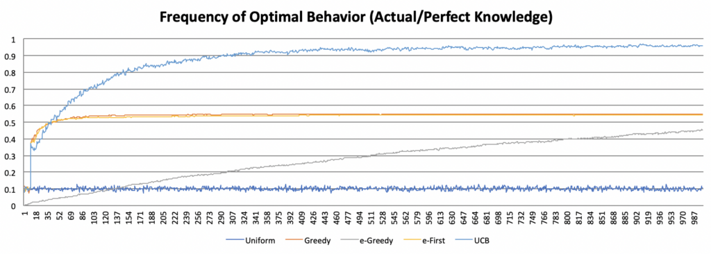
What’s interesting here is that even though the agent’s behavior is considered optimal according to the running estimate, compared with perfect knowledge of the bandits’ reward distributions, the greedy algorithm finds the highest-paying bandit only a little over 50% of the time. This result emphasizes the importance of exploration: early, randomly high-paying results can strongly influence algorithms that don’t perform adequate exploration, and yield less payoff in the long run. (Compare with the charts on page 29 of the Sutton/Barto.)
The next two algorithms are closely related in that they introduce mandatory exploration in a fixed proportion relative to the number of turns taken. This proportion, known as epsilon or e, is usually relatively small (10% or less); in my simulations, I used e = 0.01 (i.e. 1%). The e-greedy algorithm distributes the exploration uniformly across the run, while the e-first-greedy algorithm performs all of the exploration first. The graph below shows the average reward obtained for each.

As the graph illustrates, both algorithms show clear improvement over time, albeit at significantly different speeds. The e-first approach reaches a relatively high reward quickly and plateaus over the remainder of the run, while the e-greedy approach increases the reward more gradually, eventually converging with the e-first approach. Yet the cumulative reward for the e-first approach will be much higher because the agent has significantly more time to exploit the higher reward.
The final algorithm I tried was the upper confidence bound (UCB) algorithm, which balances exploration and exploitation by also taking into account the number of times a given bandit has been tested. The more a bandit has been tested, the more “confident” the algorithm becomes about its estimate, and the less valuable it is regarded for exploration. The algorithm can be customized by modifying the value placed upon exploration with the constant c. (I used c = 2 in my simulation.)

This graph shows the percentage of runs that exhibit optimal (actual) behavior with the UCB algorithm over time. The graph shows rapid improvement initially, then levels off similar to the logarithmic function. Yet this approach ultimately plateaus at a much higher level than any of the other algorithms, indicating that the UCB algorithm is effective at determining which bandit actually has the highest average payout. The graph below compares the prevalence of optimal (actual) behavior across all five algorithms.

Yet the true measure of success for the multi-armed bandit problem is the reward obtained. The following graph shows the average reward across all five algorithms.

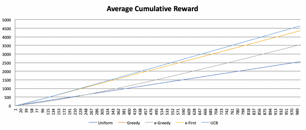
The baseline average reward represented by the uniform approach is quickly overtaken by the greedy, e-first, and UCB approaches, and more slowly by the e-greedy approach. Over time, all four algorithms converge, though the UCB is most successful. However, as discussed above, this convergence is misleading. As the UCB approach reaches its plateau very quickly, an agent using this approach will accumulate much greater rewards early on, leading to an insurmountable lead in total reward gained, even if the rates at which the rewards subsequently increase are comparable across algorithms. The chart below demonstrates this fact by comparing the average cumulative reward between approaches.

Consequently, even though the different approaches appear to converge, following the UCB approach clearly yields the greatest reward over time. Yet as Sutton and Barto point out, this result holds only for a particular kind of problem, which is in reality a simplification of the more complex problems typically encountered in the real world. Indeed, the multi-armed bandit problem is only a starting point. In future installments of this series, I will cover more advanced reinforcement learning strategies and begin to apply these strategies to the processes of musical creation.