Reinforcement Learning in Max, Part 3

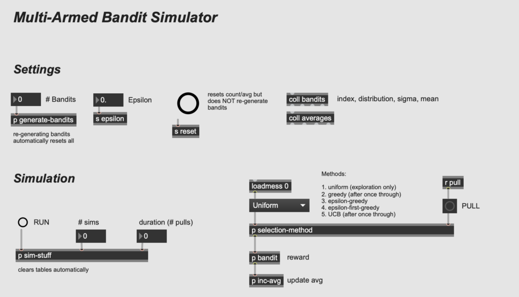
In the last post, I shared my multi-armed bandit simulator and walked through the implementation of five different reward maximization algorithms: (1) uniform, (2) greedy, (3) epsilon-greedy, (4) epsilon-first-greedy, and (5) upper confidence bound. In this post, I will present the results I obtained from my simulations, and compare those results with the trials discussed in the Sutton/Barto.

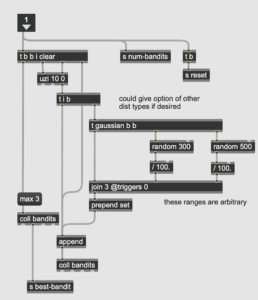
I ran 1000 simulations of each algorithm, and each simulation comprised 1000 turns. Each of the ten bandits had a different, randomly-determined reward distribution, with the mean ranging from 0.01 to 4.78, and the variance ranging from 0.66 to 2.49. I employed a Gaussian distribution for all ten bandits, using the [randdist] object.

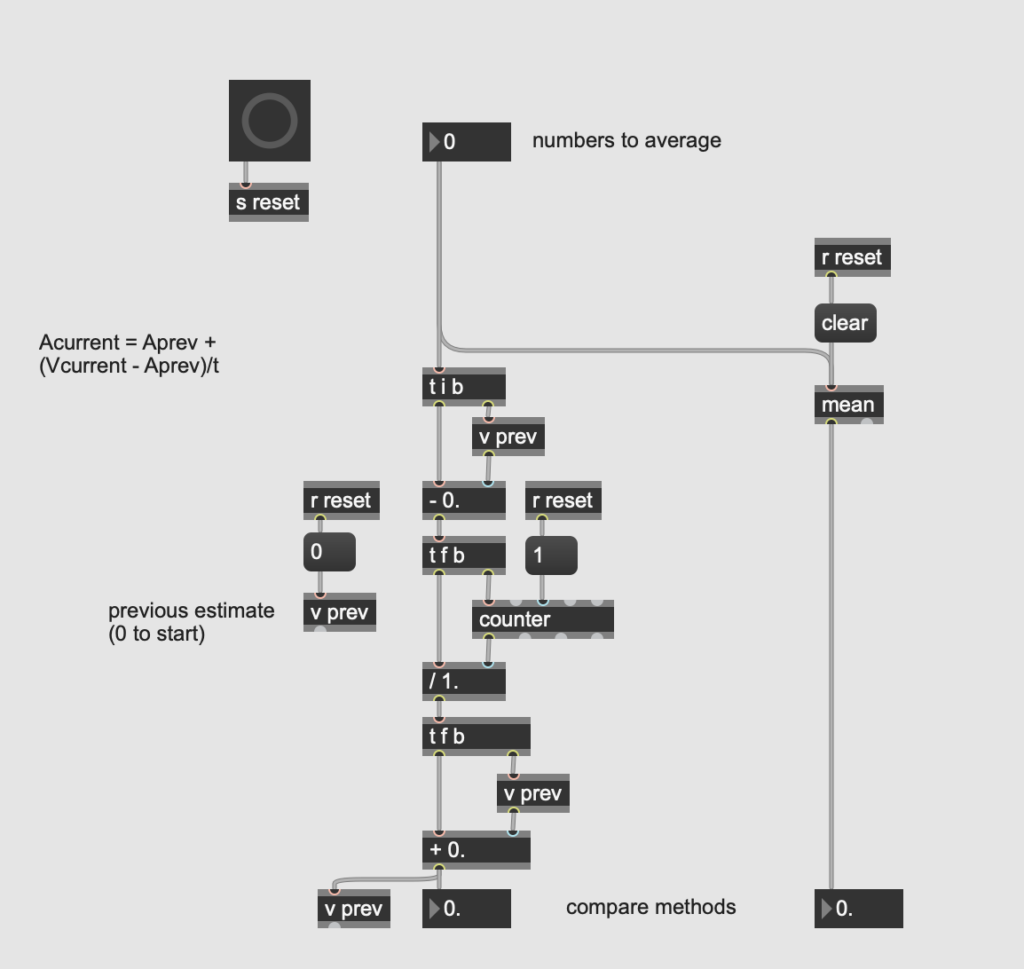
In addition to seeing which bandits were chosen in which order (and how many times)—and how their average estimates changed over time—I averaged several data points from across all of the simulations with each algorithm. The first data point was the average reward: on average, how much is gained per turn over the course of the simulation. A successful strategy would show an increase in the average reward over time through the simulation.

I also wanted to evaluate how frequently the “agent” engaged in optimal behavior. I devised two different ways to do measure that. First, I kept track of how often the agent chose the bandit with the highest average estimate. This was not necessarily the bandit with the highest average over the long term—instead, this was simply a measure of, given the available data, how frequently did the agent make the best (highest-paying) choice? The second way of evaluating this was to go by the mean of the distribution programmed into the bandit—rather than the estimate—and therefore comparing the agent’s behavior with what they might choose given perfect omniscient knowledge. I will refer to these two different measures as optimal (estimate) and optimal (actual).

My first simulation used the uniform (random) algorithm. This algorithm can be considered a kind of “control,” since it behaves exactly the same throughout the entire simulation. Since it doesn’t have a mechanism for “learning,” we don’t expect it to improve over time, as the graph of the optimal (estimate) under the uniform algorithm below shows.

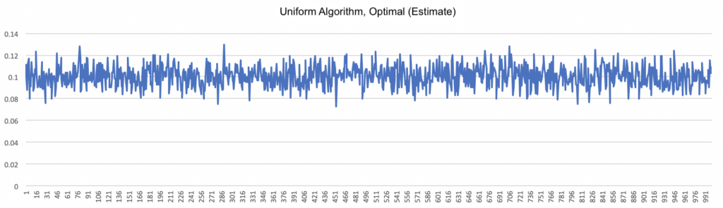
Given that there were ten bandits, if chosen at random we would expect the choice to be optimal about 10% of the time (1/10), and that is precisely what the graph shows. (As you might expect, the other graphs for the uniform algorithm are similarly static.)

By contrast, the greedy algorithm shows a marked improvement early on, but then quickly levels off. Because the greedy algorithm chooses the bandit with the highest average by definition, the optimal (estimate) graph will show optimal behavior 100% of the time (except for the brief initial exploratory period described in the previous post). More revealing is the optimal (actual) graph, given below.

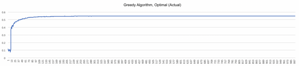
What’s interesting here is that even though the agent’s behavior is considered optimal according to the running estimate, compared with perfect knowledge of the bandits’ reward distributions, the greedy algorithm finds the highest-paying bandit only a little over 50% of the time. This result emphasizes the importance of exploration: early, randomly high-paying results can strongly influence algorithms that don’t perform adequate exploration, and yield less payoff in the long run. (Compare with the charts on page 29 of the Sutton/Barto.)

The next two algorithms are closely related in that they introduce mandatory exploration in a fixed proportion relative to the number of turns taken. This proportion, known as epsilon or e, is usually relatively small (10% or less); in my simulations, I used e = 0.01 (i.e. 1%). The e-greedy algorithm distributes the exploration uniformly across the run, while the e-first-greedy algorithm performs all of the exploration first. The graph below shows the average reward obtained for each.

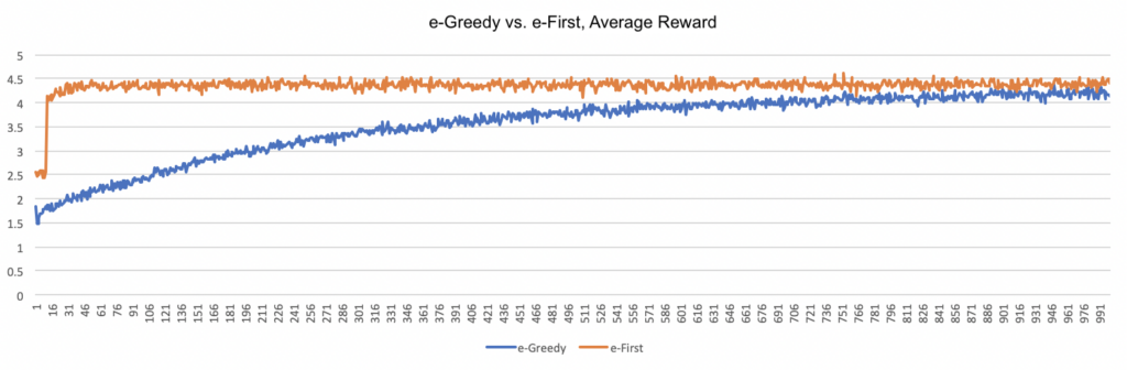
As the graph illustrates, both algorithms show clear improvement over time, albeit at significantly different speeds. The e-first approach reaches a relatively high reward quickly and plateaus over the remainder of the run, while the e-greedy approach increases the reward more gradually, eventually converging with the e-first approach. Yet the cumulative reward for the e-first approach will be much higher because the agent has significantly more time to exploit the higher reward.

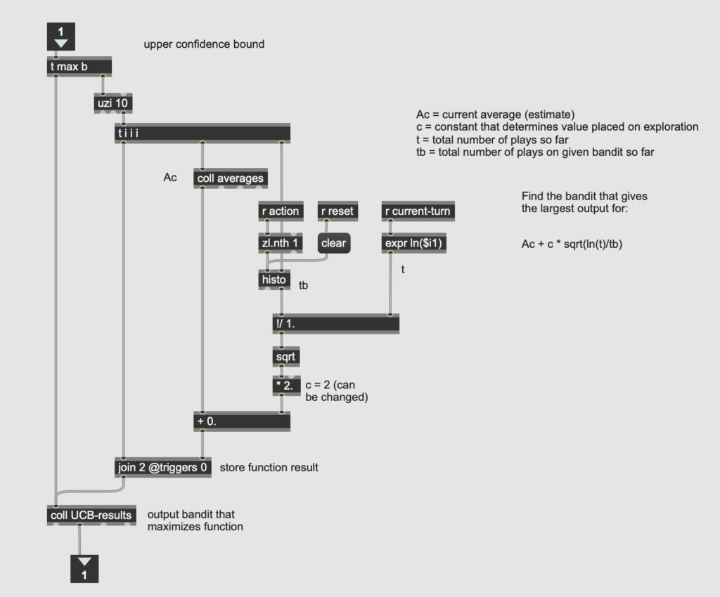
The final algorithm I tried was the upper confidence bound (UCB) algorithm, which balances exploration and exploitation by also taking into account the number of times a given bandit has been tested. The more a bandit has been tested, the more “confident” the algorithm becomes about its estimate, and the less valuable it is regarded for exploration. The algorithm can be customized by modifying the value placed upon exploration with the constant c. (I used c = 2 in my simulation.)

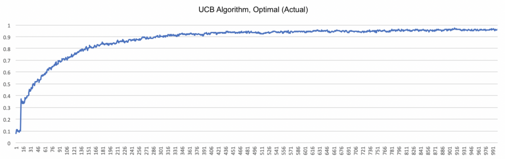
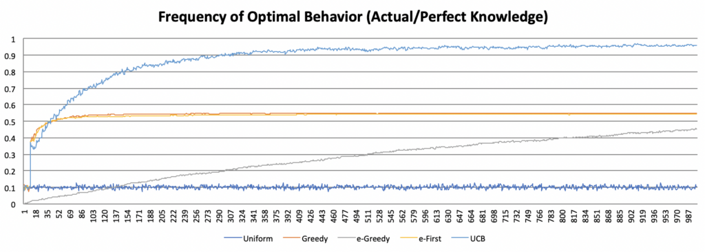
This graph shows the percentage of runs that exhibit optimal (actual) behavior with the UCB algorithm over time. The graph shows rapid improvement initially, then levels off similar to the logarithmic function. Yet this approach ultimately plateaus at a much higher level than any of the other algorithms, indicating that the UCB algorithm is effective at determining which bandit actually has the highest average payout. The graph below compares the prevalence of optimal (actual) behavior across all five algorithms.

Yet the true measure of success for the multi-armed bandit problem is the reward obtained. The following graph shows the average reward across all five algorithms.

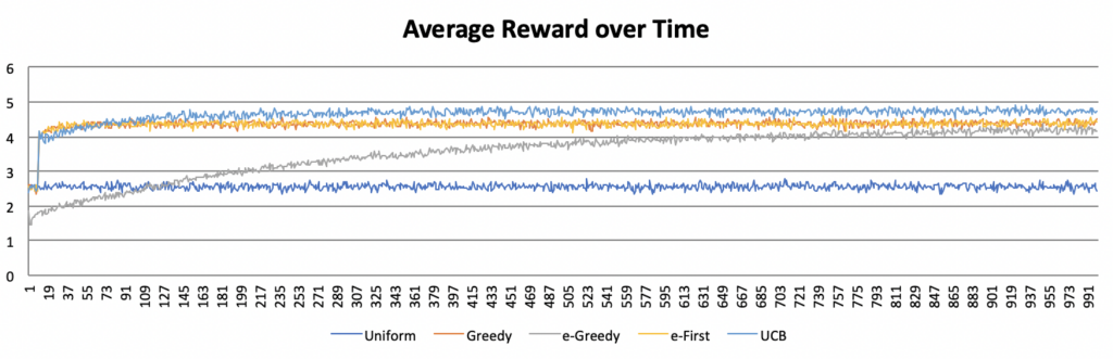
The baseline average reward represented by the uniform approach is quickly overtaken by the greedy, e-first, and UCB approaches, and more slowly by the e-greedy approach. Over time, all four algorithms converge, though the UCB is most successful. However, as discussed above, this convergence is misleading. As the UCB approach reaches its plateau very quickly, an agent using this approach will accumulate much greater rewards early on, leading to an insurmountable lead in total reward gained, even if the rates at which the rewards subsequently increase are comparable across algorithms. The chart below demonstrates this fact by comparing the average cumulative reward between approaches.

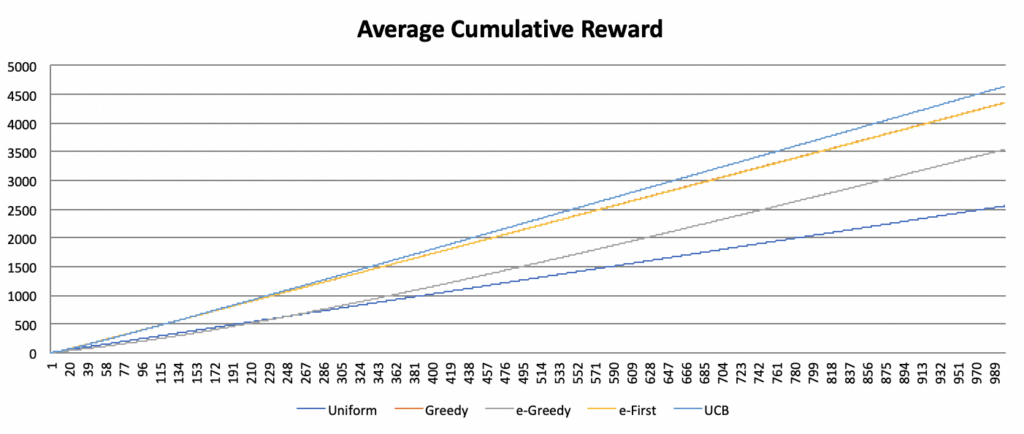
Consequently, even though the different approaches appear to converge, following the UCB approach clearly yields the greatest reward over time. Yet as Sutton and Barto point out, this result holds only for a particular kind of problem, which is in reality a simplification of the more complex problems typically encountered in the real world. Indeed, the multi-armed bandit problem is only a starting point. In future installments of this series, I will cover more advanced reinforcement learning strategies and begin to apply these strategies to the processes of musical creation.

Reinforcement Learning in Max, Part 2

In the previous post, I described the first few steps of my journey exploring reinforcement learning. In this entry, I want to share my first patch: a multi-armed bandit problem simulator. As I mentioned before, this type of problem is akin to having the opportunity to choose between many different slot machines, each with different payout distributions, with the goal of maximizing your overall payout. If you try machines at random (explore), you risk wasting time on low-paying machines; if you stick with just one or two (exploit), you risk missing out on higher-paying machines. An optimal strategy finds a balance between these two extremes.

The second chapter of the Sutton/Barto describes a few different algorithms for balancing between exploration and exploitation. It’s useful to compare different algorithms to see how well they do under different conditions. Accordingly, I wanted to build a patch that would allow me to easily switch between different algorithms. I also wanted to be able to easily run algorithms multiple times to calculate, evaluate, and compare averages over many iterations, rather than just single runs.

I started by designing the bandit generator, using the [randdist] object from the CNMAT externals package as the core. The [randdist] object allows you to specify a distribution type and variance (a.k.a. sigma, or the width of the distribution); I add an offset so that the mean for each machine is slightly different as well. The screenshot below shows the subpatch, which takes the number of bandits to be generated as input and stores the bandits (as distinct distributions defined by type, variance, and mean) in a coll object (with indices counting from zero).

Next, I built the simulation portion of the patch, which determines how many turns will be taken per simulation—how many “pulls” of the machines in total—and how many simulations. Multiple simulations are important for obtaining averages characteristic to each algorithm (plus the examples in the Sutton/Barto use multiple runs and I wanted to be able to compare my simulations with theirs). This part is quite simple—essentially one [uzi] object nested in another to keep track of the number of turns in each simulation.

After that, I built the bandit-picking portion of the patch. This involves three sub-sections: (1) defining the algorithms (and choosing one); (2) choosing a bandit and determining the reward; and (3) revising the estimate for the chosen bandit by updating the average based on the latest reward.

For the first part, I ended up implementing five different algorithms: (1) uniform; (2) greedy; (3) epsilon-greedy; (4) epsilon-first-greedy; and (5) upper confidence bound. Uniform, or pure exploration, is random throughout and so was simple to implement with a single [random] object. The greedy method, in its “pure” form, requires that the user always choose the bandit with the highest average. However, depending on the starting conditions, this could result in a single bandit being chosen for the entire simulation (e.g. if the starting “estimate” for each is zero, the first bandit pulled will give a reward greater than zero, and from here it is likely that no other bandit will ever be tested). Therefore, I chose to pull each lever once before imposing the greedy rule.

For epsilon-greedy and epsilon-first-greedy, I allow the user to choose the value for epsilon. (In my trials, I used e = 0.01.) Epsilon (e) refers to the proportion of time spent exploring at random (the proportion 1-e he gives the proportion spent being “greedy”). The difference between these two approaches is that in typical e-greedy, the exploration is randomly interspersed throughout the simulation; in e-first-greedy, the exploration occurs only at the beginning. In other words, in the former case in a simulation of 10,000 pulls with e = 0.01, 100 at random will be exploration; in the latter case, the first 100 pulls will always be exploration. It’s the same proportion, but the latter should perform slightly better because you reach your best estimates sooner and therefore have more time to exploit the best-paying machine.

The most challenging algorithm to implement was the upper confidence bound (UCB) algorithm, described in section 2.7 of the Sutton/Barto. This algorithm takes into account the number of times a given machine’s lever has been pulled, and assigns greater “confidence” to estimates with more pulls. As Sutton and Barto write, it is “better to select among the non-greedy actions according to their potential for actually being optimal” (35). A lever with fewer pulls has greater potential for a change in the average, and therefore warrants more exploration than a lever that has already been pulled many times. Just as with the greedy algorithm, I started by pulling each lever once (this is especially important here to avoid a zero in the denominator of the formula). Then I calculated the UCB algorithm for each machine on each turn, and chose the machine that optimized the algorithm (i.e. yielded the highest value).

Once a bandit was chosen, the reward was determined by loading the bandit’s properties (distribution, mean, and sigma) from the appropriate [coll] into the [randdist] object. This reward, along with the bandit index number, was then passed into the averaging formula described in the previous post to update the average estimate for the last bandit based on the most recent reward.

From here, it is possible to collect many different kinds of information about the behavior of the system. In the next post, I will discuss the output section of the patch and compare the performance of the different algorithms according to a variety of measures.

Download patch

Reinforcement Learning in Max, Part 1

This is the first entry in a series of posts dedicated to implementing reinforcement leaning algorithms in Max. Reinforcement learning is an area of machine learning I have not previously explored, so these posts will serve as both tutorials and as a way of tracking my own progress.

The idea of using a reinforcement learning strategy for a music-related machine learning project was first suggested to me by a colleague, Daniel Fox. Since it was a new area for me, I started out by doing some research. I found this library for Max, but I ultimately decided to implement the algorithms directly myself. A few especially helpful resources when getting started included:

I started out by looking at the first couple of chapters of the Sutton/Barto. I decided to begin by building a patch that could simulate a multi-armed bandit problem, since that is the problem that begins the book. A multi-armed bandit problem is a category of problem in which one is presented with a number of different options, each of which is associated with some kind of reward. The user (“the agent”) attempts to maximize the rewards gained by employing various strategies.

At the core of these problems is a tradeoff between exploration (trying unknown options) and exploitation (repeatedly making the same choice when a high reward is received). The term “multi-armed bandit” refers to a hypothetical instance of the problem in which one chooses between many different slot machines, each with different payout (reward) distributions. In this metaphor, if the agent explores too little, they may miss out on the highest-paying machine; if they explore too much, they lower their overall reward by wasting time on the low-paying machines.

As I began to read up on this problem, it became clear that I would have to lay groundwork in three major areas: (1) conceptual framing and goals; (2) mathematics; and (3) technical implementation in Max. Of the three, working out the math (and brushing off my calculus) was definitely the most difficult.

At the core of the algorithms described in the second chapter of the Sutton/Barto was the need to keep a running tally of actions taken and rewards received. This is critical for maintaining a running average for each machine, which allows the agent to determine which machine has the best payouts at each moment.

Yet as the authors point out, over the long run this approach is not computationally efficient. Instead, they introduce a formula for incrementally calculating a running average (see section 2.4), where the average is continually adjusted with each new reward, and previous rewards do not need to be stored. I found their explanation a little confusing at first, but this blog post helped clarify the formula for me. My implementation is saved as inc_avg_demo.maxpat in the download bundle.

My patch allows you to compare the incremental calculation with the results from the [mean] object. While similar in function, the [mean] object is not optimal for this application because I have to calculate an average for each of an arbitrary number of bandits. This would require an arbitrary number of [mean] objects or perpetual storage of all previous values to swap in and out (a data set that increases without limit is precisely the kind of thing we want to avoid!). My implementation can be used for multiple bandits with finite data/computation by saving the running average for each, labeling the bandit number, and using [histo], [counter] or similar to keep track of how often a given bandit has been used.

A second issue that arose was the need for random number generation following a particular distribution. While not strictly necessary, using a Gaussian (rather than uniform) distribution allowed me to more closely compare my results with those in the book. I used the [randdist] object from the CNMAT externals package (download via the Package Manager in Max).

The third issue—and the last I’ll discuss in this post—to arise in these early stages was more of a technical concern than a mathematical one. I needed to be able to receive a stream of separated data (of arbitrary length) and output it as a single list. There’s not a Max object that precisely does this: zl.group requires a number to be specified in advance, and zl.reg needs everything at once. (Incidentally, the bach.collect object does this quite nicely, but I didn’t want to invoke bach for a single operation.) I ended up creating an abstraction I call da.can (like a can, you fill it up and then dump it out) that assembles anything it receives into a list, outputs with bang, and resets with a clear message. It’s part of the collection I store here.

In my next post, I’ll share my multi-armed bandit simulator patch, which allows you to test and compare different algorithms for maximizing rewards.

Download patches