In the previous post, I described the first few steps of my journey exploring reinforcement learning. In this entry, I want to share my first patch: a multi-armed bandit problem simulator. As I mentioned before, this type of problem is akin to having the opportunity to choose between many different slot machines, each with different payout distributions, with the goal of maximizing your overall payout. If you try machines at random (explore), you risk wasting time on low-paying machines; if you stick with just one or two (exploit), you risk missing out on higher-paying machines. An optimal strategy finds a balance between these two extremes.
The second chapter of the Sutton/Barto describes a few different algorithms for balancing between exploration and exploitation. It’s useful to compare different algorithms to see how well they do under different conditions. Accordingly, I wanted to build a patch that would allow me to easily switch between different algorithms. I also wanted to be able to easily run algorithms multiple times to calculate, evaluate, and compare averages over many iterations, rather than just single runs.
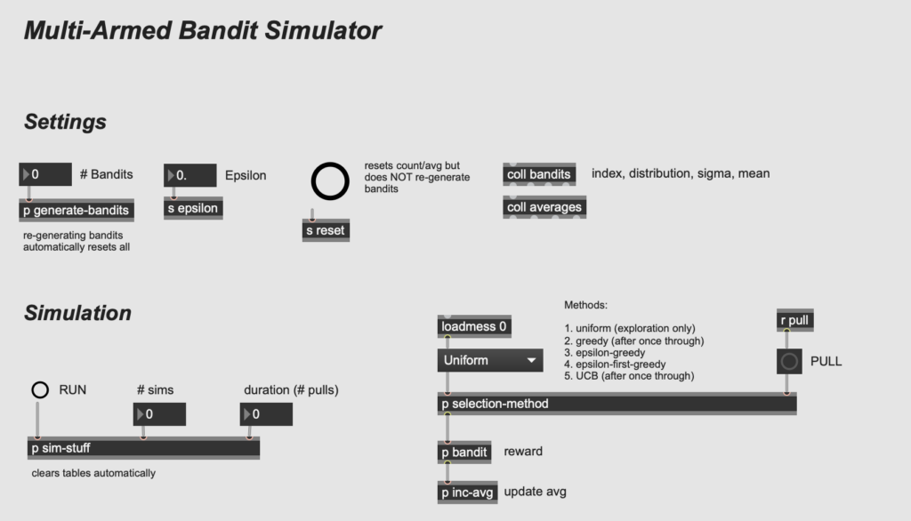
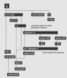
I started by designing the bandit generator, using the [randdist] object from the CNMAT externals package as the core. The [randdist] object allows you to specify a distribution type and variance (a.k.a. sigma, or the width of the distribution); I add an offset so that the mean for each machine is slightly different as well. The screenshot below shows the subpatch, which takes the number of bandits to be generated as input and stores the bandits (as distinct distributions defined by type, variance, and mean) in a coll object (with indices counting from zero).
Next, I built the simulation portion of the patch, which determines how many turns will be taken per simulation—how many “pulls” of the machines in total—and how many simulations. Multiple simulations are important for obtaining averages characteristic to each algorithm (plus the examples in the Sutton/Barto use multiple runs and I wanted to be able to compare my simulations with theirs). This part is quite simple—essentially one [uzi] object nested in another to keep track of the number of turns in each simulation.
After that, I built the bandit-picking portion of the patch. This involves three sub-sections: (1) defining the algorithms (and choosing one); (2) choosing a bandit and determining the reward; and (3) revising the estimate for the chosen bandit by updating the average based on the latest reward.
For the first part, I ended up implementing five different algorithms: (1) uniform; (2) greedy; (3) epsilon-greedy; (4) epsilon-first-greedy; and (5) upper confidence bound. Uniform, or pure exploration, is random throughout and so was simple to implement with a single [random] object. The greedy method, in its “pure” form, requires that the user always choose the bandit with the highest average. However, depending on the starting conditions, this could result in a single bandit being chosen for the entire simulation (e.g. if the starting “estimate” for each is zero, the first bandit pulled will give a reward greater than zero, and from here it is likely that no other bandit will ever be tested). Therefore, I chose to pull each lever once before imposing the greedy rule.
For epsilon-greedy and epsilon-first-greedy, I allow the user to choose the value for epsilon. (In my trials, I used e = 0.01.) Epsilon (e) refers to the proportion of time spent exploring at random (the proportion 1-e he gives the proportion spent being “greedy”). The difference between these two approaches is that in typical e-greedy, the exploration is randomly interspersed throughout the simulation; in e-first-greedy, the exploration occurs only at the beginning. In other words, in the former case in a simulation of 10,000 pulls with e = 0.01, 100 at random will be exploration; in the latter case, the first 100 pulls will always be exploration. It’s the same proportion, but the latter should perform slightly better because you reach your best estimates sooner and therefore have more time to exploit the best-paying machine.
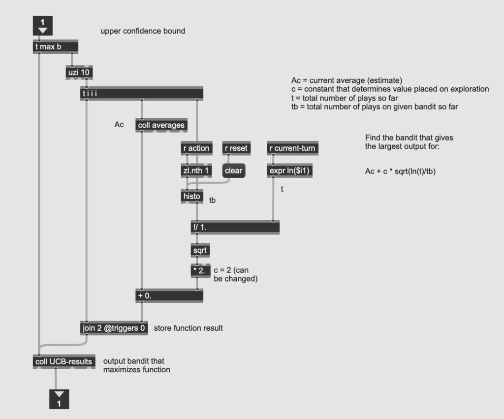
The most challenging algorithm to implement was the upper confidence bound (UCB) algorithm, described in section 2.7 of the Sutton/Barto. This algorithm takes into account the number of times a given machine’s lever has been pulled, and assigns greater “confidence” to estimates with more pulls. As Sutton and Barto write, it is “better to select among the non-greedy actions according to their potential for actually being optimal” (35). A lever with fewer pulls has greater potential for a change in the average, and therefore warrants more exploration than a lever that has already been pulled many times. Just as with the greedy algorithm, I started by pulling each lever once (this is especially important here to avoid a zero in the denominator of the formula). Then I calculated the UCB algorithm for each machine on each turn, and chose the machine that optimized the algorithm (i.e. yielded the highest value).
Once a bandit was chosen, the reward was determined by loading the bandit’s properties (distribution, mean, and sigma) from the appropriate [coll] into the [randdist] object. This reward, along with the bandit index number, was then passed into the averaging formula described in the previous post to update the average estimate for the last bandit based on the most recent reward.
From here, it is possible to collect many different kinds of information about the behavior of the system. In the next post, I will discuss the output section of the patch and compare the performance of the different algorithms according to a variety of measures.